|
1
|
- MS Computer Science Thesis Defense
|
|
2
|
- Phylogenetics
- Neural Networks
- SOTA
- KomPhy
- Results
- Birth-death trees
- Uniform trees
- Comparison with other algorithms
- Parallel Implementation
|
|
3
|
|
|
4
|
|
|
5
|
- Neural networks were inspired by the conception of neurons in the brain
being very simple computational devices which, when linked together in
interesting ways, are able to learn.
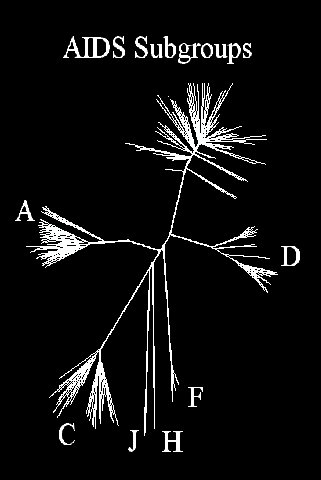
- Each neuron performs a simple calculation on its input and generates
output.
- Neuron output flows from neuron to neuron until an output neuron is
reached.
- Can produce approximate solutions to complex problems very quickly.
|
|
6
|
- State Space Search
- NP-Hard (Graham and Foulds, 1982)
- Phylogenetics is a process of inference from uncertain and incomplete
evidence.
- Heuristics and approximate solutions are welcome for large data sets.
|
|
7
|
- Each output neuron has an associated weight vector.
- Each component of the weight vector modulates a component of the input
vector.
|
|
8
|
- A particular input from an input set is mapped onto the input neurons.
- As each new input is presented to the network an output neuron becomes
associated with it (wins).
- The winning neuron is made more likely to win again given the same
input.
- In this way the network learns to recognize classes of input by
associating each neuron with a subset of the input set.
|
|
9
|
- The competitive neural network has two components.
- is a member of the input set
- Ri is
- Max net equivalent to argmax( Ri )
|
|
10
|
- Once a winning neuron has been determined the learning rule is applied
to it.
|
|
11
|
- The weight vectors associated with each neuron can be thought of as
points in a weight space.
- Since they are of the same dimensionality as the weights the inputs can
also be mapped into weight space.
|
|
12
|
- Element 1 of input set S is presented to the network.
- The distance (dot product) between
and
- S1 is calculated.
|
|
13
|
- is found to be closer to S1
and the learning rule is applied to it.
|
|
14
|
- is found to be closer to S1
and the learning rule is applied to it.
- becomes more like S1
|
|
15
|
- S2 is presented to the network.
- is found to be closer to S2
and the learning rule is applied to it.
|
|
16
|
- S2 is presented to the network.
- is found to be closer to S2
and the learning rule is applied to it.
- becomes more like S2
|
|
17
|
- S3 is presented to the network.
- is found to be closer to S3
and the learning rule is applied to it.
|
|
18
|
- S3 is presented to the network.
- is found to be closer to S3
and the learning rule is applied to it.
- becomes more like S3
|
|
19
|
- S4 is presented to the network.
- is found to be closer to S4
and the learning rule is applied to it.
|
|
20
|
- S4 is presented to the network.
- is found to be closer to S4
and the learning rule is applied to it.
- becomes more like S4
|
|
21
|
- S5 is presented to the network.
- is found to be closer to S5
and the learning rule is applied to it.
|
|
22
|
- S5 is presented to the network.
- is found to be closer to S5
and the learning rule is applied to it.
- becomes more like S5
|
|
23
|
- S6 is presented to the network.
- is found to be closer to S6
and the learning rule is applied to it.
|
|
24
|
- S6 is presented to the network.
- is found to be closer to S6
and the learning rule is applied to it.
- becomes more like S6
|
|
25
|
- S7 is presented to the network.
- is found to be closer to S7
and the learning rule is applied to it.
|
|
26
|
- S7 is presented to the network.
- is found to be closer to S7
and the learning rule is applied to it.
- becomes more like S7
|
|
27
|
- S6 is presented to the network.
- is found to be closer to S6
and the learning rule is applied to it.
- becomes more like S6
|
|
28
|
- The set of input vectors is typically presented to the network numerous
times. Each cycle of presentations is called an epoch.
- Various methods can be used to determine when to finish training the
network and output the partitions:
- Root Mean Squared (RMS) error between weights and sequences.
- Fixed number of epochs.
|
|
29
|
- The number of epochs required for the network to converge depends on α
in the learning rule and the distances between input vectors.
- The smaller α is the more training cycles are needed for the
neurons to reach a stable point in weight space.
- Large α values can cause the network to converge quickly but if
they are too large the neurons may get stuck in an unstable cycle.
|
|
30
|
- In 1997 Dopazo J. and J. M. Carazo published a paper in the Journal of
Molecular Evolution describing a neural network approach to phylogeny
reconstruction they called SOTA.
- SOTA employs a Self Organizing Network (SOM) to reconstruct phylogenies.
- SOMs use some of the same concepts as competitive neural networks.
|
|
31
|
- The main difference between a SOM and a competitive network is that in
the SOM numerous neurons are embedded in a large mesh.
- The neurons are divided up into neighborhoods (many local maxnets) and
go though cycles of inhibition and excitation.
- The mesh determines the excitatory and inhibitory relationships.
- After some number of cycles the neurons congregate in the weight space
in such a way that they map out areas of high probability.
|
|
32
|
- Dopazo and Corazo’s paper describes the reconstruction of two
phylogenies both of which are real data sets for which the true tree is
unknown.
- SOTA and related SOMs were adapted to perform protein sequence
clustering and function prediction but none of the follow up papers deal
with phylogenetic reconstruction specifically [2][3].
- There is a need for more analysis of neural network approaches to
phylogeny reconstruction.
|
|
33
|
- Top-down divide-and-conquer algorithm
- Constructive (could be faulted for not providing alternative trees)
- The algorithm partitions the input sequences into two at each recursive
step
- The partitioning is done by a two node Kohonen competitive neural
network
|
|
34
|
- Distances between weights and input sequences can be calculated using
available phylogenetic methods
- These methods must be modified to accept real numbered distances between
characters
- Euclidian distance provides a good approximation for parsimony
- Jukes-Cantor, Tanamura-Nei, and F84 were adapted for KomPhy
- Unfortunately the initial weight to input distances are too great for
F84 and Tanamua-Nei
|
|
35
|
- Each base is represented by an apex of this regular tetrahedron.
- Weight components transition smoothly from base to base as points within
this volume.
|
|
36
|
|
|
37
|
|
|
38
|
|
|
39
|
|
|
40
|
|
|
41
|
|
|
42
|
- That speciation events result in two populations which are equally able
to generate new speciation events.
- That is, subtrees tend to be
balanced.
- Poor assumption since the subtree sizes depend as much on selection bias
of the researcher as on the evolutionary history.
|
|
43
|
|
|
44
|
|
|
45
|
|
|
46
|
|
|
47
|
|
|
48
|
|
|
49
|
|
|
50
|
|
|
51
|
|
|
52
|
|
|
53
|
|
|
54
|
|
|
55
|
|
|
56
|
|
|
57
|
|
|
58
|
- Joshua Leiderberg (DENRAL):
- “It is easy to sympathize with computer scientists who are willing to
rely on neural-network approaches that ignore, may even defeat, insight
into causal relationships.”
- (Foreword, AI and Molecular Biology, 1992)
- “One of the most difficult steps in development of an expert system is
the exploitation of domain wizards. Therein may lie the greatest
hazards from the proliferation of expert systems: for much of that
expert knowledge is fallible.”
- (Afterword, AI and Mol. Biol. 1992)
|
|
59
|
- KomPhy provides a point of comparison to the previous neural network
approach.
- about as accurate as SOTA (worse on uniform trees and better on
birth-death trees).
- faster than SOTA.
- Not as good or as fast as existing algorithms such as neighbor-joining
- Both neural network approaches show a strong bias towards generating
balanced trees so they do poorly on uniform trees
|
|
60
|
- Tanamura-Nei and F84 distances were used with KomPhy but were unable to
converge the network because the weights and inputs are initially too
far apart.
- Other sophisticated distances (such as K2P) should be tried.
- KomPhy supports the creation of n-fircatating trees with neurons
dynamically added at each recursive step. Experiments are needed to
determine the utility of this feature.
- Branches could be labeled with lengths derived from the distances
between neurons at the previous recursive step.
|

 Notes
Notes